Gradient Descent implementation in Python

During my learning time, I came across one awesome channel which helped me a lot to understand and implement. I believe watching helps one retain better than just reading, so I am going to leave that link here.

Implementation will be done on Python as the title suggests and the dataset is a teeny tiny one that is used in the code basics video given above, you can get it here.

So let's start with importing the libraries we need. Pandas, NumPy, and matplotlib are all we need. After importing them, upload the data.

We will implement all three gradient descent. The first implementation will be of Batch Gradient Descent. Before we define the function of GD, we have to scale the features.

Why scaling?

You can see that area, bedroom, and price are three different features. So to make them come all in unison we have to scale them. Scaling will help to range the values between 0 and 1. We will use MinMax Scaler () to scale the data.

After scaling the data, we will define the function of Gradient descent:

def gradient_descent(x,y,epochs, learning_rate=0.01):
        number_of_features=x.shape[1]     
        w = np.ones(shape=(number_of_features))#weights
        b=0 #bias
        total_samples= x.shape[0] # number of rows in X

The number of features will be 2 so that's what we are setting in. W is weights and b is bias. The formula we are using :

Total_samples is the number of records we have in our dataset.

cost_list=[]
epoch_list=[]

We will also declare two lists that will capture our cost and epoch so we can plot a graph to see what's happening:

for i in range(epochs):
y_pred=np.dot(w, x.T) + b

# this is same as y=mx+b. [xT] is transpose of x
# Next step is derivative. This formula can be taken in as it is or you can go ahead and indulge yourself in deep maths.

w_grad = -(2/total_samples)*(x.T.dot(y-y_pred))
b_grad = -(2/total_samples)*np.sum(y-y_pred)

# Second step is to adjust the weights using derivative

w = w — learning_rate * w_grad
b = b — learning_rate * b_grad

#cost is mean squared error

cost=np.mean(np.square(y-y_pred))

#We need to save the cost and epoch value of some iterations so we can plot the graph. We will go with every 10th value. The values will get added to the cost and epoch list we made

if i %10==0:
cost_list.append(cost)
epoch_list.append(i)

#Return the weight, bias , cost list, and epoch list

return w, b, cost, cost_list, epoch_list

>> Now we will call the function we made:

w, b, cost, cost_list, epoch_list = gradient_descent(scaled_x,scaled_y.reshape(scaled_y.shape[0],),500)

w, b, cost

Your output will look something like this:

(array([0.70712464, 0.67456527]), -0.23034857438407427, 0.0068641890429808105)

i.e. w1 is 0.7071, w2 is 0.6745 and bias is -0.2303

Now we need to define one 'predict' function for our BGD:

def predict(Area,Bedroom,w,b):
scaled_X = sx.transform([[Area, Bedroom]])[0]

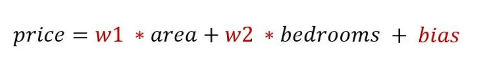
# here w1 = w[0] , w2 = w[1], and bias is b
# equation for price is w1*area + w2*bedrooms + bias
# scaled_X[0] is area
# scaled_X[1] is bedroom

scaled_price = w[0] * scaled_X[0] + w[1] * scaled_X[1] + b

# once we get price prediction we need to to rescal it back to original value
# also since it returns 2D array, to get single value we need to do value[0][0]if you don't add it your price will come with 2 sets of brackets

return sy.inverse_transform([[scaled_price]])[0][0]

#we will predict price for 2600 sq ft and 4 bedroom house:

predict(2600,4,w,b)
128.45484403267596

close enough!. I think you would like to see the graph for which we saved cost and epoch. To print a graph:

plt.xlabel(“epoch”)
plt.ylabel(“cost”)
plt.plot(epoch_list,cost_list)

The function for stochastic and mini is almost the same with just a little bit of adjustment. For stochastic, we will use random to select a random sample from the dataset.

#We will import random
import random
def SGD(X, y_true, epochs, learning_rate = 0.01):
     number_of_features = X.shape[1]
# numpy array with 1 row and columns equal to the number of features.
# In our case number_of_features = 2(area, bedroom )
w = np.ones(shape=(number_of_features))
b = 0
total_samples = X.shape[0]

cost_list = []
epoch_list = []

for i in range(epochs):
     random_index = random.randint(0,total_samples-1)
# random index from total samples
sample_x = X[random_index]
sample_y = y_true[random_index]

y_predicted = np.dot(w, sample_x.T) + b

w_grad = -(2/total_samples)*(sample_x.T.dot(sample_y-y_predicted))
b_grad = -(2/total_samples)*(sample_y-y_predicted)

w = w — learning_rate * w_grad
b = b — learning_rate * b_grad

cost = np.square(sample_y-y_predicted)

if i%100==0: # at every 100th iteration record the cost and epoch value
cost_list.append(cost)
epoch_list.append(i)

return w, b, cost, cost_list, epoch_list
w_sgd, b_sgd, cost_sgd, cost_list_sgd, epoch_list_sgd = SGD(scaled_x,scaled_y.reshape(scaled_y.shape[0],),10000)
w_sgd, b_sgd, cost_sgd

The graph will look something like this:

Mini Batch has one more argument in its function which is the number of batches.

def mini_batch_gradient_descent(X, y_true, epochs = 100, batch_size = 5, learning_rate = 0.01):
number_of_features = X.shape[1]
w = np.ones(shape=(number_of_features))
b = 0
total_samples = X.shape[0]
if batch_size > total_samples: # In this case mini batch becomes same as batch gradient descent
batch_size = total_samples

cost_list = []
epoch_list = []

num_batches = int(total_samples/batch_size)

for i in range(epochs):
random_indices = np.random.permutation(total_samples)
X_tmp = X[random_indices]
y_tmp = y_true[random_indices]

for j in range(0,total_samples,batch_size):
Xj = X_tmp[j:j+batch_size]
yj = y_tmp[j:j+batch_size]
y_predicted = np.dot(w, Xj.T) + b

w_grad = -(2/len(Xj))*(Xj.T.dot(yj-y_predicted))
b_grad = -(2/len(Xj))*np.sum(yj-y_predicted)

w = w — learning_rate * w_grad
b = b — learning_rate * b_grad

cost = np.mean(np.square(yj-y_predicted)) # MSE (Mean Squared Error)

if i%10==0:
cost_list.append(cost)
epoch_list.append(i)

return w, b, cost, cost_list, epoch_list
w, b, cost, cost_list, epoch_list = mini_batch_gradient_descent(scaled_x,scaled_y.reshape(scaled_y.shape[0],),epochs = 120,batch_size = 5)
w, b, cost

So with this, we have completed the implementation of all three gradient descent algorithms with their plots. I hope I was able to make it understandable for you guys. Like this and help to spread the love.

Happy coding!! :)